Introduction to lighthouse.codebook • lighthouse.codebook

Creating codebooks

Creating a codebook involves two general steps:

Create a “codebook” object in R from a data frame (and, optionally, metadata), using cb_create() or a specialized variant (such as cb_create_spss() or cb_create_redcap()).
Write the codebook to disk using cb_write().

library(lighthouse.codebook)

# create and write a codebook without metadata
dat |> 
  cb_create() |> 
  cb_write("cb.xlsx")

# with metadata
dat |> 
  cb_create(metadata = dat1_metadata) |> 
  cb_write("cb.xlsx")

# from SPSS data
dat_spss <- haven::read_sav("dat_spss.sav", user_na = TRUE)

dat_spss |> 
  cb_create_spss() |> 
  cb_write("cb_spss.xlsx")

# from REDCap data
dat_rc <- REDCapR::redcap_read(redcap_uri = rc_uri, token = rc_token)
meta_rc <- REDCapR::redcap_metadata_read(redcap_uri = rc_uri, token = rc_token)

dat_rc$data |> 
  cb_create_redcap(metadata = meta_rc$data) |> 
  cb_write("cb_rc.xlsx")

Codebook contents

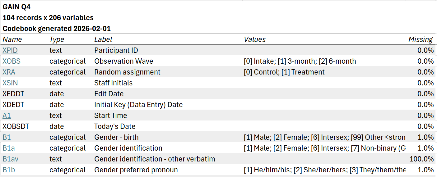
The codebook written to disk will include an overview tab listing all variables in the dataset; summary tabs for numeric, categorical, and text variables; and, if grouping variables are specified, grouped summary tabs for numeric and categorical variables.

The overview tab includes one row for each variable in the dataset, with information on variable types, labels, values, and missingness. By default, each variable is hyperlinked to its location on the relevant summary tab.

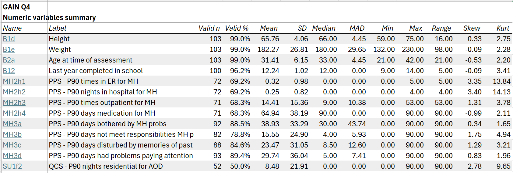
The numeric summary tab includes descriptive statistics for all numeric variables in the dataset:

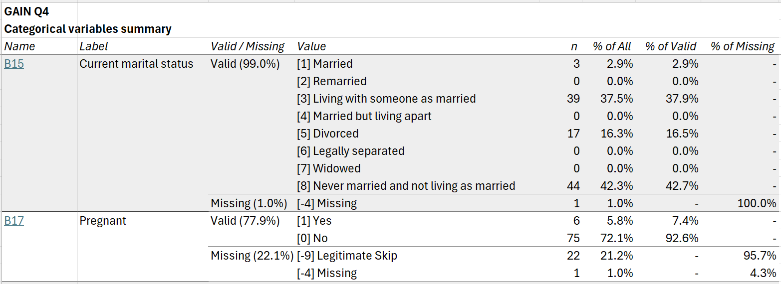
The categorical summary tab includes frequencies for all categorical variables, optionally with separate rows for user missing values:

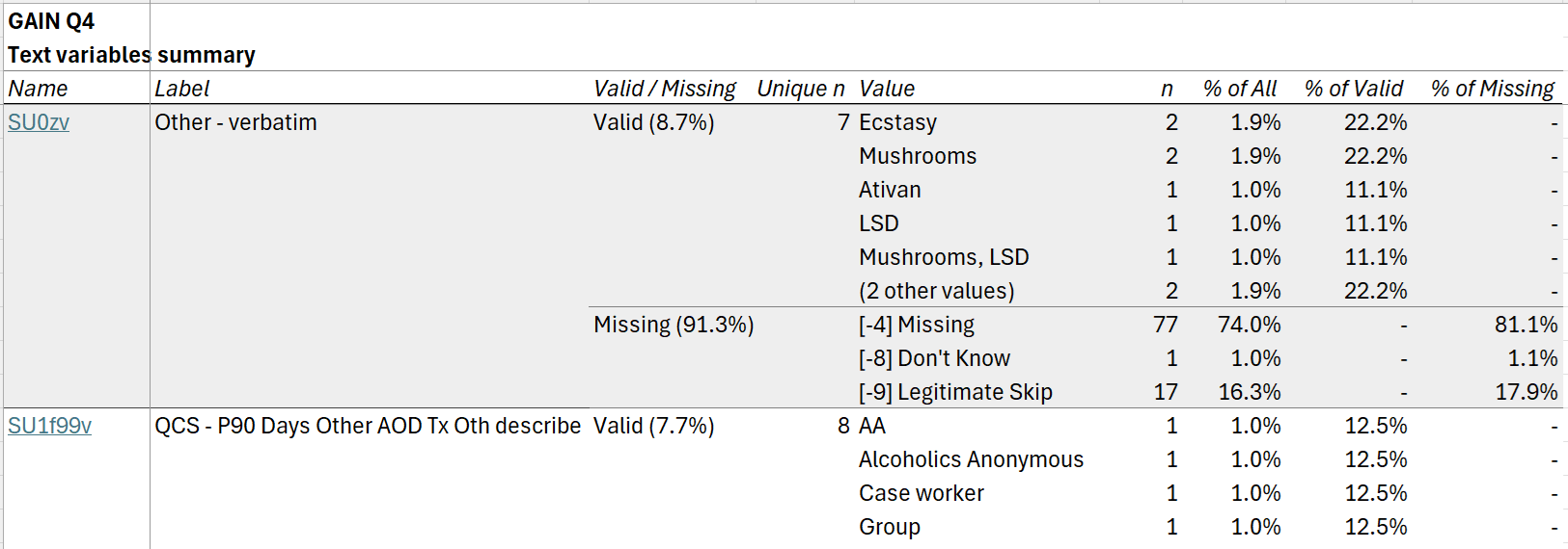
Finally, the text summary tab includes frequencies for the most common values for all text variables in the dataset. (The number of values shown can be adjusted using the n_text_vals argument to cb_write().)

If group_by is specified in cb_write(), additional numeric and categorical summary tabs grouped by the specified variables will be included.

Customizing codebooks

There are many options for controlling how data is interpreted, summarized, and presented. This section shows a few of the most useful options. Further options are detailed in the documentation for cb_create() and cb_write().

Grouped summaries

Numeric and categorical data summaries can be grouped by one or more variables by specifying them in the group_by argument to cb_write().

cb_create(data, metadata) |>
  cb_write("cb.xlsx", group_by = treatment_group)

cb_create(data, metadata) |>
  cb_write("cb.xlsx", group_by = c(treatment_group, timepoint, age_group))

By default, values for each subgroup are shown in separate columns, with decked heads if more than one grouping variable is specified. However, some or all grouping variables can instead be shown in rows using the group_rows argument.

# show `treatment_group` in columns and `timepoint` in rows
cb_create(data, metadata) |>
  cb_write(
    "cb.xlsx", 
    group_by = c(treatment_group, timepoint),
    group_rows = timepoint
  )

Different row grouping behavior can be specified for numeric versus categorical summary tabs using the group_rows_numeric and group_rows_categorical arguments.

# for numeric summary, show `treatment_group` in columns and `timepoint` in rows;
# for categorical summary, show all grouping variables in columns
cb_create(data, metadata) |>
  cb_write(
    "cb.xlsx", 
    group_by = c(treatment_group, timepoint),
    group_rows_numeric = timepoint
  )

# for numeric summary, show all grouping variables in rows; 
# for categorical summary, show `treatment_group` in rows
cb_create(data, metadata) |>
  cb_write(
    "cb.xlsx", 
    group_by = c(treatment_group, timepoint),
    group_rows_numeric = c(treatment_group, timepoint),
    group_rows_categorical = treatment_group
  )

User missing values

User missing values (also known as nonresponse codes, reserve codes, or special values) can be specified using the .user_missing argument to cb_create(). Missing values are specified using a formula or list of formulas, with variables on the left-hand side (as names or tidyselect expressions) and values on the right-hand side. If the left-hand side is empty, user missings will be set for all compatible variables in the dataset.

# set a single missing value for a single variable
cb <- cb_create(data, metadata, .user_missing = var1 ~ 99)

# for variables `var1` through `var5`
cb <- cb_create(data, metadata, .user_missing = var1:var5 ~ c(98, 99))

# for all numeric variables, plus `var6` and `var7`
cb <- cb_create(
  data, 
  metadata, 
  .user_missing = c(where(is.numeric), var6, var7) ~ c(-9, -8, -7)
)

# for all compatible variables in dataset
cb <- cb_create(data, metadata, .user_missing = ~ c(98, 99))

If the user missing values are named, the names will be treated as value labels in data summaries.

cb <- cb_create(
  data, 
  metadata, 
  .user_missing = var1:var5 ~ c("Declined" = 98, "Not applicable" = 99)
)

To apply different user missings for different variables, pass a list of formulas.

cb <- cb_create(
  data, 
  metadata,
  .user_missing = list(
    starts_with("status") ~ c("Declined" = 98, "Not applicable" = 99),
    var7:var10 ~ c("Don't know" = -4, "Not applicable" = -5)
  )
)

Missing value handling

On numeric summary tabs, missing values (including both user missing values and NA) are dropped for computation of summary statistics.

On ungrouped categorical and text summary tabs, by default, user missing values are individually tabulated. For example, if .user_missing = ~ c("Declined" = 98, "Not applicable" = 99), then categorical and text summary tabs will include rows giving counts for "[98] Declined" and "[99] Not applicable". All user missing values and NA can instead be collapsed into a single "(Missing)" row using the detail_missing argument to cb_write().

dat |>
  cb_create(.user_missing = ~  ~ c("Declined" = 98, "Not applicable" = 99)) |>
  cb_write("cb.xlsx", detail_missing = FALSE)

Finally, user missing values are always collapsed (as though detail_missing = FALSE) on grouped summary tabs.

Splitting long variable labels

Variable labels for sets of related variables sometimes share a common prefix. Using the .split_var_labels argument to cb_create(), this prefix can be extracted into a separate column, making it easier to see at a glance what is unique about each variable.

For example, given a set of variable labels that all begin with "What colors do you like? Select all that apply: ":

Name	Label
age	How old are you today?
colors1	What colors do you like? Select all that apply: Red
colors2	What colors do you like? Select all that apply: Green
colors3	What colors do you like? Select all that apply: Blue
colors4	What colors do you like? Select all that apply: Orange
height	What is your height in inches?

You can split the labels for these variables, specifying them using a tidyselect expression:

cb_create(
    data, 
    metadata, 
    .split_var_labels = starts_with("colors")
  ) |>
  cb_write("cb.xlsx")

Name	Label Stem	Label
age		How old are you today?
colors1	What colors do you like? Select all that apply:	Red
colors2	What colors do you like? Select all that apply:	Green
colors3	What colors do you like? Select all that apply:	Blue
colors4	What colors do you like? Select all that apply:	Orange
height		What is your height in inches?

Multiple sets of variables with common prefixes can be specified by passing a list of tidyselect expressions.

cb_create(
    data, 
    metadata, 
    .split_var_labels = list(
      starts_with("colors"), 
      fav_food2:fav_food9, 
      c(rating1, rating4:rating7, rating9)
    )
  ) |>
  cb_write("cb.xlsx")

Variable typing

Data summaries are produced for “numeric,” “categorical,” and “text” variables. For a given variable x, * x is treated as categorical if (1) it is a factor, ordered factor, or logical vector, or (2) it has associated value labels other than missing value codes (specified in metadata or, for SPSS data, in a "haven_labelled" vector). * x is treated as numeric if (1) it is numeric (i.e., is.numeric(x) is TRUE) and (2) it has no associated value labels other than missing value codes. * x is treated as text if (1) it is a character vector and (2) it has no associated value labels other than missing value codes.

Thus, you can change how a variable is summarized by changing its class. For instance, to get complete frequencies for a numeric or character variable, convert it to a factor; to get only the top frequencies for a factor with many levels, convert it to character.

Variables of other classes, such as dates, datetimes, and lists, are not currently included on summary tabs. Summaries for dates and datetimes are planned for a future release.

Other uses for the codebook object

The "lighthouse_codebook" object created by cb_create() will most commonly be used to write an Excel codebook to disk using cb_write(). However, it can also be used to create other objects in R.

# example data
q4_subset <- gain_q4 |> 
  subset(select = c(XPID, XOBS, XRA, B17, SU4a, SU4b, SU1f99v))

# create codebook
cb <- cb_create(
  q4_subset,
  metadata = q4_metadata,
  .user_missing =  ~ c("Not Asked" = -3, 
                      "Missing" = -4, 
                      "Confidential" = -6, 
                      "Refused" = -7,
                      "Don't Know" = -8, 
                      "Legitimate Skip" = -9)
)

cb
# # A tibble: 7 × 6
#   name    type        label                         values user_missings missing
#   <chr>   <chr>       <chr>                         <chr>  <chr>           <dbl>
# 1 XPID    text        Participant ID                NA     [-9] Legitim…   0
# 2 XOBS    categorical Observation Wave              [0] I… [-9] Legitim…   0
# 3 XRA     categorical Random assignment             [0] C… [-9] Legitim…   0
# 4 B17     categorical Pregnant                      [0] N… [-9] Legitim…   0.221
# 5 SU4a    numeric     PPS - P90 days alcohol use    NA     [-9] Legitim…   0.394
# 6 SU4b    numeric     PPS - P90 days drunk or 5+ d… NA     [-9] Legitim…   0.442
# 7 SU1f99v text        QCS - P90 Days Other AOD Tx … NA     [-9] Legitim…   0.923

Extract transformed data

Use cb_get_data() to extract transformed data based in several formats. format = "factors" yields a dataset with all variables with value labels converted to factors and user missings converted to NA.

cb_get_data(cb, format = "factors")
# # A tibble: 104 × 7
#    XPID  XOBS    XRA       B17    SU4a  SU4b SU1f99v       
#    <chr> <fct>   <fct>     <fct> <dbl> <dbl> <chr>
#  1 001   Intake  Treatment No       NA    NA NA
#  2 002   Intake  Control   No       10     4 NA
#  3 003   Intake  Treatment No       10     1 Peer counselor
#  4 003   3-month Treatment No       39    15 NA
#  5 003   6-month Treatment No       NA    NA NA
#  6 004   Intake  Control   No       10     2 NA
#  7 004   3-month Control   No       55    63 NA
#  8 004   6-month Control   No       10     1 NA
#  9 005   Intake  Control   Yes      35     0 Social worker
# 10 005   3-month Control   Yes      55    39 NA
# # ℹ 94 more rows

Whereas format = "haven" yields a dataset with SPSS-style variable labels, value labels, and user missings encoded using the "haven_labelled_spss" class.

cb_get_data(cb, format = "haven")
# # A tibble: 104 × 7
#    XPID      XOBS        XRA           B17       SU4a      SU4b      SU1f99v    
#    <chr+lbl> <dbl+lbl>   <dbl+lbl>     <dbl+lbl> <dbl+lbl> <dbl+lbl> <chr+lbl>
#  1 001       0 [Intake]  1 [Treatment] 0 [No]    -9 (NA)   -9 (NA)   -9 (NA)    
#  2 002       0 [Intake]  0 [Control]   0 [No]    10         4        -9 (NA)    
#  3 003       0 [Intake]  1 [Treatment] 0 [No]    10         1        Peer couns…
#  4 003       1 [3-month] 1 [Treatment] 0 [No]    39        15        -4 (NA)
#  5 003       2 [6-month] 1 [Treatment] 0 [No]    -4 (NA)   -4 (NA)   -4 (NA)
#  6 004       0 [Intake]  0 [Control]   0 [No]    10         2        -9 (NA)    
#  7 004       1 [3-month] 0 [Control]   0 [No]    55        63        -9 (NA)
#  8 004       2 [6-month] 0 [Control]   0 [No]    10         1        -9 (NA)
#  9 005       0 [Intake]  0 [Control]   1 [Yes]   35         0        Social wor…
# 10 005       1 [3-month] 0 [Control]   1 [Yes]   55        39        -9 (NA)
# # ℹ 94 more rows

Get data summaries

cb_summarize_numeric(), cb_summarize_categorical(), and cb_summarize_text() return summaries for all variables of their respective types. These are the basis of the summary tabs generated by cb_write().

cb_summarize_numeric(cb)
# # A tibble: 2 × 8
#   name  label                         valid_n valid_pct  mean    SD median   MAD
#   <chr> <chr>                           <int>     <dbl> <dbl> <dbl>  <dbl> <dbl>
# 1 SU4a  PPS - P90 days alcohol use         63     0.606 23.4   21.2     20 25.2 
# 2 SU4b  PPS - P90 days drunk or 5+ d…      58     0.558  8.09  13.6      2  2.97
# # ℹ 5 more variables: min <dbl>, max <dbl>, range <dbl>, skew <dbl>, kurt <dbl>

cb_summarize_categorical(cb) |> 
# # A tibble: 9 × 7
#   name  label             is_missing value             n pct_of_all pct_of_valid
#   <chr> <chr>             <lgl>      <chr>         <int>      <dbl>        <dbl>
# 1 XOBS  Observation Wave  FALSE      [0] Intake       42    0.404         0.404
# 2 XOBS  Observation Wave  FALSE      [1] 3-month      34    0.327         0.327
# 3 XOBS  Observation Wave  FALSE      [2] 6-month      28    0.269         0.269
# 4 XRA   Random assignment FALSE      [0] Control      50    0.481         0.481 
# 5 XRA   Random assignment FALSE      [1] Treatment    54    0.519         0.519
# 6 B17   Pregnant          FALSE      [1] Yes           6    0.0577        0.0741
# 7 B17   Pregnant          FALSE      [0] No           75    0.721         0.926
# 8 B17   Pregnant          TRUE       [-9] Legitim…    22    0.212        NA
# 9 B17   Pregnant          TRUE       [-4] Missing      1    0.00962      NA     
# # ℹ 1 more variable: pct_of_missing <dbl>

cb_summarize_text(cb)
# # A tibble: 14 × 7
#    name    label                      is_missing unique_n value     n pct_of_all
#    <chr>   <chr>                      <lgl>         <int> <chr> <int>     <dbl>
#  1 XPID    Participant ID             FALSE            42 003       3    0.0288 
#  2 XPID    Participant ID             FALSE            42 004       3    0.0288
#  3 XPID    Participant ID             FALSE            42 005       3    0.0288
#  4 XPID    Participant ID             FALSE            42 006       3    0.0288
#  5 XPID    Participant ID             FALSE            42 010       3    0.0288
#  6 XPID    Participant ID             FALSE            42 (37 …    89    0.856
#  7 SU1f99v QCS - P90 Days Other AOD … FALSE             8 AA        1    0.00962
#  8 SU1f99v QCS - P90 Days Other AOD … FALSE             8 Alco…     1    0.00962
#  9 SU1f99v QCS - P90 Days Other AOD … FALSE             8 Case…     1    0.00962
# 10 SU1f99v QCS - P90 Days Other AOD … FALSE             8 Group     1    0.00962
# 11 SU1f99v QCS - P90 Days Other AOD … FALSE             8 NA        1    0.00962
# 12 SU1f99v QCS - P90 Days Other AOD … FALSE             8 (3 o…     3    0.0288 
# 13 SU1f99v QCS - P90 Days Other AOD … TRUE             NA [-4]…    44    0.423
# 14 SU1f99v QCS - P90 Days Other AOD … TRUE             NA [-9]…    52    0.5
# # ℹ 2 more variables: pct_of_valid <dbl>, pct_of_missing <dbl>

cb_summarize_numeric() and cb_summarize_categorical() can also return grouped summaries:

cb_summarize_numeric(cb, group_by = XOBS)
# # A tibble: 6 × 8
#   XOBS    name  label                      valid_n valid_pct  mean     SD median
#   <fct>   <chr> <chr>                        <int>     <dbl> <dbl>  <dbl>  <dbl>
# 1 Intake  SU4a  PPS - P90 days alcohol use      30     0.714 28.8  20.1     26.5
# 2 3-month SU4a  PPS - P90 days alcohol use      20     0.588 21.4  21.0     12.5
# 3 6-month SU4a  PPS - P90 days alcohol use      13     0.464 13.9  21.5      6
# 4 Intake  SU4b  PPS - P90 days drunk or 5…      30     0.714  7.13 10.7      4
# 5 3-month SU4b  PPS - P90 days drunk or 5…      15     0.441 16.1  20.0      3
# 6 6-month SU4b  PPS - P90 days drunk or 5…      13     0.464  1     0.707    1
# # ℹ 6 more variables: MAD <dbl>, min <dbl>, max <dbl>, range <dbl>, skew <dbl>, 
# #   kurt <dbl>

cb_summarize_categorical(cb, group_by = XRA)
# # A tibble: 12 × 7
#    XRA       name  label            value           n pct_of_all pct_of_valid
#    <fct>     <chr> <chr>            <chr>       <int>      <dbl>        <dbl>
#  1 Control   XOBS  Observation Wave [0] Intake     20     0.4          0.4
#  2 Control   XOBS  Observation Wave [1] 3-month    16     0.32         0.32  
#  3 Control   XOBS  Observation Wave [2] 6-month    14     0.28         0.28
#  4 Treatment XOBS  Observation Wave [0] Intake     22     0.407        0.407
#  5 Treatment XOBS  Observation Wave [1] 3-month    18     0.333        0.333
#  6 Treatment XOBS  Observation Wave [2] 6-month    14     0.259        0.259
#  7 Control   B17   Pregnant         [1] Yes         3     0.06         0.0811
#  8 Control   B17   Pregnant         [0] No         34     0.68         0.919 
#  9 Control   B17   Pregnant         (Missing)      13     0.26        NA
# 10 Treatment B17   Pregnant         [1] Yes         3     0.0556       0.0682
# 11 Treatment B17   Pregnant         [0] No         41     0.759        0.932
# 12 Treatment B17   Pregnant         (Missing)      10     0.185       NA